[8]:

import h5py
import matplotlib.pyplot as plt

Explore the options used in the solver

[11]:

with h5py.File('./hdf5/H2_adf_dzp_QMCTorch.hdf5', 'r') as f5:
    print(f5['Solver'].keys())

<KeysViewHDF5 ['cuda', 'hdf5file', 'opt', 'qmctorch_version', 'sampler', 'save_model', 'wf']>

[12]:

with h5py.File('./hdf5/H2_adf_dzp_QMCTorch.hdf5', 'r') as f5:
    print(f5['Solver']['wf'].keys())

<KeysViewHDF5 ['ao', 'atoms', 'configs', 'configs_method', 'cuda', 'fc', 'gradients', 'highest_occ_mo', 'include_all_mo', 'jastrow', 'jastrow_type', 'kinetic', 'kinetic_energy', 'kinetic_method', 'mo', 'mol', 'natom', 'nci', 'ndim', 'ndim_tot', 'nelec', 'nmo_opt', 'orb_confs', 'pool', 'training', 'use_backflow', 'use_jastrow']>

[16]:

with h5py.File('./hdf5/H2_adf_dzp_QMCTorch.hdf5', 'r') as f5:
    print(f5['Solver']['wf']['configs_method'][()])

b'single_double(2,2)'

Explore the results of the wave function optimization

[17]:

with h5py.File('./hdf5/H2_adf_dzp_QMCTorch.hdf5', 'r') as f5:
    print(f5['wf_opt'].keys())

<KeysViewHDF5 ['ao.bas_exp', 'energy', 'fc.weight', 'geometry', 'jastrow.jastrow_kernel.weight', 'local_energy', 'mo.mo_modifier', 'models', 'qmctorch_version']>

[18]:

with h5py.File('./hdf5/H2_adf_dzp_QMCTorch.hdf5', 'r') as f5:
    det_weigts = f5['wf_opt']['fc.weight'][()]

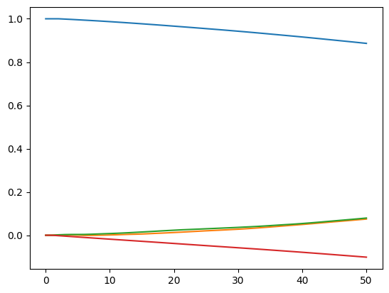
[19]:

plt.plot(det_weigts.squeeze())

[19]:

[<matplotlib.lines.Line2D at 0x743fd87eddc0>,
 <matplotlib.lines.Line2D at 0x743fd87ede20>,
 <matplotlib.lines.Line2D at 0x743fd87ede50>,
 <matplotlib.lines.Line2D at 0x743fd87edf40>]

../_images/notebooks_12_Explore_results_8_1.png

[ ]: